Table of Contents
List of Figures
- 1.1. Coordinate system.
- 1.2. Vector image
- 1.3. Raster image
- 1.4. Sampling grid
- 1.5. Sample depth
- 1.6. RGB bands
- 1.7. Indexed image
- 1.8. Run-length encoding
- 1.9. JPEG generation loss
- 2.1. Screenshot of gluas
- 2.2. basic gluas program
- 3.1. histogram
- 3.2. chromaticity diagram
- 3.3. luminance profile
- 4.1. threshold
- 4.2. brightness
- 4.3. brightness subtraction
- 4.4. contrast
- 4.5. brightness and contrast
- 4.6. invert
- 4.7. gamma
- 4.8. The GIMP's levels tool
- 4.9. levels
- 4.10. The GIMP's curves tool
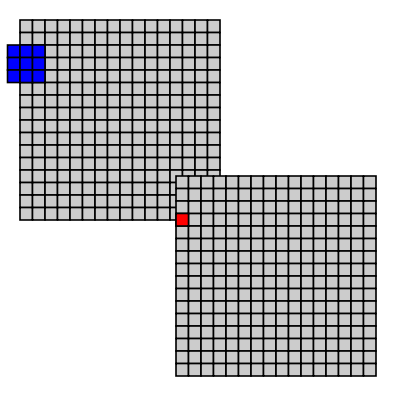
- 5.1. Sliding window
- 5.2. Over the edge
- 5.3. convolve
- 5.4. blur
- 5.5. kuwahara
- 5.6. median
- 5.7. jitter
- 6.1. translation
- 6.2. rotation
- 6.3. scaling
- 6.4. bilinear
- 6.5. bicubic
- 6.6. box decimate
- 7.1. contrast stretching
- 7.2. grayworld assumption
- 7.3. component stretching
- 7.4. ace
List of Tables
Colophon
“ Recursivly look for new association when association fails during naming of a method or class. ”
This text was written according to the DocBook XML DTD. Both manually using vim, and through custom ruby scripts.
![[Tip]](images/tip.png) | Printing |
|---|---|
If you need to print the entire document, use the single xhtml output image_processing.xhtml. FireFox is known to provide a nice print-out using the CSS applied. | |
xsltproc, db2latex pdftex and latex-ucs are used to generate the PDF version , while xsltproc and Norman Walsh's XSL stylesheets are used for the XHTML version. (validate)
The typographical layout is done with a CSS stylesheet tailored to the very well structured docbook hierarchy of classes. This stylesheet could serve as a starting point for other docbook stylesheets since it has good layout, decorations, color and image use seperation.
![[Caution]](images/caution.png) | Caution |
|---|---|
The XHTML CSS2 stylesheet doesn't work fully with Internet Explorer, but should degrade gracefully. The main remaining problem seems to be able to set the width of the body element of a webpage. | |
For figures dealing with images and extraction of data from images, figures with accompanying code is shown, when shown in a webbrowser the images linked are the actual pixel by pixel image data.
The afore mentioned figures, the output of image processing algorithms, are autogenerated XML docbook fragments, changing a line in a lua script, will trigger a change that makes The GIMP run in batch mode to duplicate the image, apply lua script with gluas, extend image size, shift layer and save as a new png file. The detection of a new png image will trigger a rebuild of an xml fragment that can be included with an XML entity. In short editing a lua file, updates the rendered pdf and html views. It saves a lot of typing to have this set up, a lot of mundane work being done in the background.
The other graphics was prepared using The GIMP, cairo/rcairo and ImageMagick's convert.
This text has been written in various places, Gjøvik, Oslo, Berlin and Brussels.
![[Note]](images/note.png) | Note to Developers/Writers |
|---|---|
This document can be seen as a collaborative effort, patches are welcome. New algorithms and/or a port to nickle would be most welcome. | |
“The rays, to speak properly, are not colored; in them there is nothing else than a certain power and disposition to stir up a sensation of this or that color.”
This text tries to teach the art of digitally alter and conjure images to your own liking. It attempts doing so from a programming mind set instead of a mathematical one. Becoming intimate with a colored sampling grid is the ultimate goal of it.
The text concentrates on the aspects used by filters, but the skills presented are also applicable to computer graphics and ray tracing. OpenGL and hardware acceleration have removed some of the center stage in the world of computer graphics, the revenge over the origamic geometries will come from a more sampling oriented world, with surfels; voxels reborn.
“Virtual image, a point or system of points, on one side of a mirror or lens, which, if it existed, would emit the system of rays which actually exists on the other side of the mirror or lens.”
One way to describe an image using numbers is to declare its contents using position and size of geometric forms and shapes like lines, curves, rectangles and circles; such images are called vector images.
We need a coordinate system to describe an image, the coordinate system used to place elements in relation to each other is called user space, since this is the coordinates the user uses to define elements and position them in relation to each other.
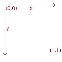
The coordinate system used for all examples in this document has the origin in the upper left, with the x axis extending to the right and y axis extending downwards.
It would have been nice to make a smiling face, instead of the dissatisfied face on the left, by using a bezier curve, or the segment of a circle this could be achieved, this being a text focusing mainly on raster graphics though, that would probably be too complex.
A simple image of a face can be declared as follows:
Figure 1.2. Vector image
draw circle
     center        0.5, 0.5
     radius        0.4
     fill-color    yellow
     stroke-color  black
     stroke-width  0.05
draw circle
     center        0.35, 0.4
     radius        0.05
     fill-color    black
draw circle
     center        0.65, 0.4
     radius        0.05
     fill-color    black
draw line
     start         0.3, 0.6
     end           0.7, 0.6
     stroke-color  black
     stroke-width  0.1

The preceding description of an image can be seen as a “cooking recipe” for how to draw the image, it contains geometrical primitives like lines, curves and cirles describing color as well as relative size, position and shape of elements. When preparing the image for display is has to be translated into a bitmap image, this process is called rasterization.
A vector image is resolution independent, this means that you can enlarge or shrink the image without affecting the output quality. Vector images are the preferred way to represent Fonts, Logos and many illustrations.
Bitmap-, or raster [1] -, images are “digital photographs”, they are the most common form to represent natural images and other forms of graphics that are rich in detail. Bitmap images is how graphics is stored in the video memory of a computer. The term bitmap refers to how a given pattern of bits in a pixel maps to a specific color.
| Note |
|---|---|
In the other chapters of introduction to image molding, raster images is the only topic. | |
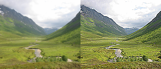
Figure 1.3. Raster image
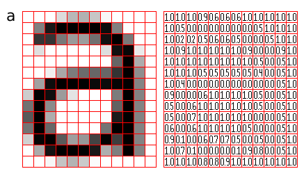
A bitmap images take the form of an array, where the value of each element, called a pixel picture element, correspond to the color of that portion of the image. Each horizontal line in the image is called a scan line.
The letter 'a' might be represented in a 12x14 matrix as depicted in Figure 3., the values in the matrix depict the brightness of the pixels (picture elements). Larger values correspond to brighter areas whilst lower values are darker.
When measuring the value for a pixel, one takes the average color of an area around the location of the pixel. A simplistic model is sampling a square, this is called a box filter, a more physically accurate measurement is to calculate a weighted Gaussian average (giving the value exactly at the pixel coordinates a high weight, and lower weight to the area around it). When perceiving a bitmap image the human eye should blend the pixel values together, recreating an illusion of the continuous image it represents.
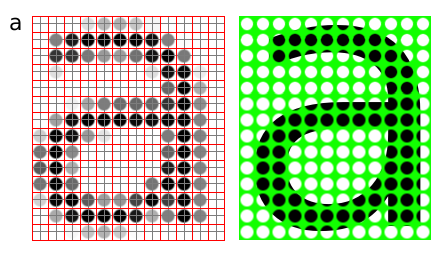
The number of horizontal and vertical samples in the pixel grid is called Image dimensions, it is specified as width x height.
Resolution is a measurement of sampling density, resolution of bitmap images give a relationship between pixel dimensions and physical dimensions. The most often used measurement is ppi, pixels per inch [2].
Figure 1.4. Sampling grid
Megapixels refer to the total number of pixels in the captured image, an easier metric is image dimensions which represent the number of horizontal and vertical samples in the sampling grid. An image with a 4:3 aspect ratio with dimension 2048x1536 pixels, contain a total of 2048x1535=3,145,728 pixels; approximately 3 million, thus it is a 3 megapixel image.
Table 1.1. Common image dimensions
| Dimensions | Megapixels | Name | Comment |
|---|---|---|---|
| 640x480 | 0.3 | VGA | VGA |
| 720x576 | 0.4 | CCIR 601 DV PAL | Dimensions used for PAL DV, and PAL DVDs |
| 768x576 | 0.4 | CCIR 601 PAL full | PAL with square sampling grid ratio |
| 800x600 | 0.4 | SVGA | |
| 1024x768 | 0.8 | XGA | The currently (2004) most common computer screen dimensions. |
| 1280x960 | 1.2 | ||
| 1600x1200 | 2.1 | UXGA | |
| 1920x1080 | 2.1 | 1080i HDTV | interlaced, high resolution digital TV format. |
| 2048x1536 | 3.1 | 2K | Typically used for digital effects in feature films. |
| 3008x1960 | 5.3 | ||
| 3088x2056 | 6.3 | ||
| 4064x2704 | 11.1 |
When we need to create an image with different dimensions from what we have we scale the image. A different name for scaling is resampling, when resampling algorithms try to reconstruct the original continous image and create a new sample grid.
The process of reducing the image dimensions is called decimation, this can be done by averaging the values of source pixels contributing to each output pixel.
When we increase the image size we actually want to create sample points between the original sample points in the original raster, this is done by interpolation the values in the sample grid, effectivly guessing the values of the unknown pixels[3].
The values of the pixels need to be stored in the computers memory, this means that in the end the data ultimately need to end up in a binary representation, the spatial continuity of the image is approximated by the spacing of the samples in the sample grid. The values we can represent for each pixel is determined by the sample format chosen.
Figure 1.5. Sample depth
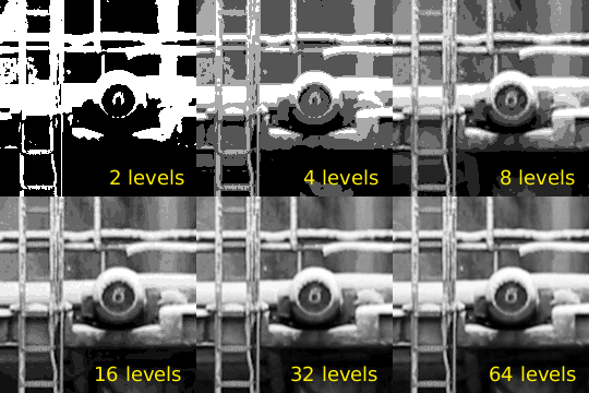
A common sample format is 8bit integers, 8bit integers can only represent 256 discrete values (2^8 = 256), thus brightness levels are quantized into these levels.
For high dynamic range images (images with detail both in shadows and highlights) 8bits 256 discrete values does not provide enough precision to store an accurate image. Some digital cameras operate with more than 8bit samples internally, higher end cameras (mostly SLRs) also provide RAW images that often are 12bit (2^12bit = 4096).
The PNG and TIF image formats supports 16bit samples, many image processing and manipulation programs perform their operations in 16bit when working on 8bit images to avoid quality loss in processing, the film industry in Hollywood often uses floating point values to represent images to preserve both contrast, and information in shadows and highlights.
The most common way to model color in Computer Graphics is the RGB color model, this corresponds to the way both CRT monitors and LCD screens/projectors reproduce color. Each pixel is represented by three values, the amount of red, green and blue. Thus an RGB color image will use three times as much memory as a gray-scle image of the same pixel dimensions.
Figure 1.6. RGB bands
One of the most common pixel formats used is 8bit rgb where the red, green and blue values are stored interleaved in memory. This memory layout is often referred to as chunky, storing the components in seperate buffers is called planar, and is not as common.
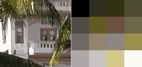
It was earlier common to store images in a palletized mode, this works similar to a paint by numbers strategy. We store just the number of the palette entry used for each pixel. And for each palette entry we store the amount of red, green and blue light.
Bitmap images take up a lot of memory, image compression reduces the amount of memory needed to store an image. For instance a 2.1 megapixel, 8bit RGB image (1600x1200) occupies 1600x1200x3 bytes = 5760000 bytes = 5.5 megabytes, this is the uncompressed size of the image.
Compression ratio is the ratio between the compressed image and the uncompressed image, if the example image mentioned above was stored as a 512kb jpeg file the compression ratio would be 0.5mb : 5.5mb = 1:11.
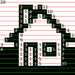
When an image is losslessly compressed, repetition and predictability is used to represent all the information using less memory. The original image can be restored. One of the simplest lossless image compression methods is run-length encoding. Run-length encoding encodes consecutive similar values as one token in a data stream.
Figure 1.8. Run-length encoding
70,
5, 25,
5, 27,
4, 26,
4, 25,
6, 24,
6, 23,
3, 2, 3, 22,
3, 2, 3, 21,
3, 5, 2, 20,
3, 5, 2, 19,
3, 7, 2, 18,
3, 7, 2, 17,
14, 16,
14, 15,
3, 11, 2, 14,
3, 11, 2, 13,
3, 13, 2, 12,
3, 13, 2, 11,
3, 15, 2, 10,
3, 15, 2, 8,
6, 12, 6, 6,
6, 12, 6, 64
In Figure 1.8, “Run-length encoding” a black and white image of a house has been compressed with run length encoding, the bitmap is considered as one long string of black/or white pixels, the encoding is how many bytes of the same color occur after each other. We'll further reduce the amount of bytes taken up by these 72 numerical values by having a maximum span length of 15, and encoding longer spans by using multiple spans separated by zero length spans of the other color.
70,                     15,  0, 15,  0, 15,  0, 10,
 5, 25,                  5, 15,  0, 10,
 5, 27,                  6, 15,  0, 12,
 4, 26,                  4, 15,  0, 11,
 4, 25,                  4, 15,  0, 10,
 6, 24,                  6, 15,  0,  9,
 6, 23,                  6, 15,  0,  8,
 3,  2, 3, 22,           3,  2,  3, 15,  0,  7,
 3,  2, 3, 21,           3,  2,  3, 15,  0,  6,
 3,  5, 2, 20,           3,  5,  2, 15,  0,  5,
 3,  5, 2, 19,           3,  5,  2, 15,  0,  4,
 3,  7, 2, 18,           3,  7,  2, 15,  0,  3,
 3,  7, 2, 17,           3,  7,  2, 15,  0,  2
14, 16,                 14, 15,  0,  1
14, 15,                 14, 15,
 3, 11, 2, 14,           3, 11,  2, 14,
 3, 11, 2, 13,           3, 11,  2, 13,
 3, 13, 2, 12,           3, 13,  2, 12,
 3, 13, 2, 11,           3, 13,  2, 11,
 3, 15, 2, 10,           3, 15,  2, 10,
 3, 15, 2,  8,           3, 15,  2,  8,
 6, 12, 6,  6,           6, 12,  6,  6,
 6, 12, 6, 64            6, 12,  6, 15, 0, 15, 0, 15, 0, 15, 0, 4
The new encoding is 113 nibbles long, a nibble i 4bit and can represent the value 0--4, thus we need 57 bytes to store all our values, which is less than the 93 bytes we would have needed to store the image as a 1bit image, and much less than the 750 bytes needed if we used a byte for each pixel. Run length encoding algorithms used in file formats would probably use additional means to compress the RLE stream achieved here.
Lossy image compression takes advantage of the human eyes ability to hide imperfection and the fact that some types of information are more important than others. Changes in luminance are for instance seen as more significant by a human observer than change in hue.
JPEG is a file format implementing compression based on the Discrete Cosine Transform DCT, together with lossless algorithms this provides good compression ratios. The way JPEG works is best suited for images with continuous tonal ranges like photographs, logos, scanned text and other images with lot's of sharp contours / lines will get more compression artifacts than photographs.
Lossy compression algorithms should not be used as a working format, only final copies should be saved as jpeg since loss accumulates over generations.
Figure 1.9. JPEG generation loss
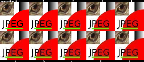
An image specially constructed to show the deficiencies in the JPEG compression algorithm, saved, reopened and saved again 9 times.
JPEG is most suited for photographics content where the adverse effect of the compression algorithm is not so evident.
JPEG is not suited as an intermediate format, only use JPEG for final distribution where filesize actually matters.
Many applications have their own internal file format, while other formats are more suited for interchange of data. Table ref# lists some of the most common image formats.
Table 1.2. Vector File Formats
| Extension | Name | Notes |
|---|---|---|
| .ai | Adobe Illustrator Document | Native format of Adobe Illustrator (based on .eps) |
| .eps | Encapsulated Postscript | Industry standard for including vector graphics in print |
| .ps | PostScript | Vector based printing language, used by many Laser printers, used as electronic paper for scientific purposes. |
| Portable Document Format | Modernized version of ps, adopted by the general public as 'electronic print version' | |
| .svg | Scalable Vector Graphics | XML based W3C standard, incorporating animation, gaining adoption. |
| .swf | Shockwave Flash | Binary vector format, with animation and sound, supported by most major web browsers. |
Table 1.3. Raster File Formats
| Extension | Name | Notes |
|---|---|---|
| .gif | Graphics Interchange Format | 8bit indexed bitmap format, is superceded by PNG on all accounts but animation |
| .jpg | Joint Photographic Experts Group | Lossy compression format well suited for photographic images |
| .png | Portable Network Graphics | Lossless compression image, supporting 16bit sample depth, and Alpha channel |
| .tiff, .tif | Tagged Image File Format | |
| .psd | Photoshop Document | Native format of Adobe Photoshop, allows layers and other structural elements |
| .raw, .raw | Raw image file | Direct memory dump from a digital camera, contains the direct imprint from the imaging sensor, before bayer interpolation and other color corrections. |
| .xcf | Gimp Project File | GIMP's native image format. |
[1] raster n: formation consisting of the set of horizontal lines that is used to form an image on a CRT
[2] The difference between ppi and dpi, is the difference between pixels and dots - pixels can represent multiple values, whilst a dot is a monochrome spot of ink or toner of a single colorant as produced by a printer. Printers use a process called half toning to create a monochrome pattern the simulates a range of intensity levels.
[3] When using the digital zoom of a camera, the camera is using interpolating to guess the values that are not present in the image. Capturing an image at the maximum analog zoom level, and doing the post processing of cropping and rescaling on the computer will give equal or better results.
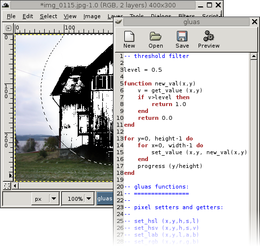
Gluas is a gimp plug-in providing a enviroment for testing algorithms for image processing. The environment contains a simple editor for entering the algorithms. It uses the lua interpreter.
Gluas can be downloaded from Gluas download page, to be able to use gluas properly you also need an installation of The GIMP.
| Note |
|---|---|
Note that the author doesn't know the windows installation procedure in detail. Any contribution to clarify would be welcome. | |
The gluas installer on the website provides for a system wide installation of gluas, this is the easiest way to install gluas,
| Caution |
|---|---|
If The GIMP has been installed in a location where the user does not have write privileges, you need to do a per user install. | |
Procedure 2.1. Installing gluas from source
Preqrequisites
You need The GIMP's developer files (headers), as well as an installed lua runtime, with development files (headers). In Debian™ the following packages, and their dependencies need to be installed:
- liblua50
- liblua50-dev
- liblualib50
- liblualib50-dev
- gimp
- libgimp2.0
- libgimp2.0-dev
For syntax highlighting libgtksourceview must be installed as well.
Download
The latest release of the gluas source can be found in the files subfolder of the gluas website. The latest version is the version with the highest version number, at the time of writing that was 0.1.19.
At the commandline, entering:
wget http://pippin.gimp.org/plug-ins/gluas/files/gluas-0.1.19.tar.gz
should be sufficient to complete this step, although checking for a never version using a web browser is recommended.
Extract
tar xvzf gluas-0.1.19.tar.gz
The characters after the command tar indicates what the tar applications should do, the meaning of the used characters are:
- x
extract
- v
verbose
- z
ungzip (uncompress, replace this with j, for .tar.bz2 files)
- f
the input to tar is a file (as opposed to data coming on standard input)
Enter the gluas directory
cd gluas-0.1.19
Configure
./configure
This will prepare compilation of the gluas plug-in for your specific system, if any components/packages that are needed are not found, the configure script will complain.
Tip Running configure takes a little while, prepare a cup of tea while it runs.
Make
make
Compiling gluas should not take a long time, the binary produced can either be manually placed in the users private plug-in folder, or be installed systemwide.
Relax If you are following the previous tip, you can now drink your tea.
Install
We need to be the super user to install the application, thus we need to become root.
su
Password: joshua
Caution If you already are root, ask someone who knows why this is stupid.
Now we issue the command to do the actual installation of our compiled program.
make install
The next time you start the Gimp, gluas should be available from the menu system at: ->->.
The enviroment set up when processing starts, sets the global variables width and height, functions for setting and getting pixels are provided
A programming tutorial for lua is out of scope for this document, the samples given elsewhere in this document should provide a feel for the language, some peculiarities of lua is explained here, look at The lua website, for a short overview when reading sample code Lua Short Reference might come in handy.
There are functions to set and get individual pixels, they are of the form:
v get_value(x, y);
set_value(x, y, v);
See the section called “Gluas reference” for more functions, and details.
All values used in gluas are floating point values, unless mandated by the color model, the normal range is from 0.0 to 1.0. This range is used instead of an more arbitary range like 0-255, 0-42, 0-100 or 0-65535.
The width and height of the image in pixels can be accessed through global variables with those names.
The GIMP takes care of modifying only the portions that are part of the current selection, as well as blending old and new pixel values for partially selected pixels.
The coordinates of the boundingbox of the selection can be accessed through global variables, see bound_x0, bound_y0 and bound_x1, bound_y1.
When pixels are set, they don't immediatly overwrite the original pixel values. This is to facilitate area operations. When multipass algorithms are implemented, like a two pass blur, the changes can be comitted to the source buffer by issuing
A mischellaneus collections of samples reside at The gluas gallery. As well as part of the work in progress Images Processing using gluas.
In the following sample the code needed for a simple thresholding filter is documented.
Figure 2.2. basic gluas program
for y=0, height-1 do
  for x=0, width-1 do
    v = get_value (x,y)

    if v < 0.5 then
       v=1.0
    else
       v=0.0
    end

    set_value (x,y,v)
  end
  progress (y/height)
end
By either pressing the button with gears, or pressing F5 gluas will apply the algorihm described. If any processing errors occur an error panel will appear at the top of the gluas window.
Gluas uses the core lua language for processing, but extends it with some functions specific to interaction with The GIMP.
r,g,b,a get_rgba(x, y);
Returns the Red, Green, Blue and Alpha components for the coordinates specified by the x,y parameters. The values are taken from the source image which is the original pixel data, unless flush() has been invoked.
RGB values within gluas are values between 0.0 and 1.0.
set_rgba(x, y, r, g, b, a);
Sets a pixel, using the specified Red, Green, Blue and Alpha component values.
r,g,b get_rgb(x, y);
set_rgb(x, y, r, g, b);
Functions similar to the RGBA varieties, note that the set_rgb function will not preserve the alpha value of the pixel, but boost it to 1.0 (full opacity).
h,s,l get_hsl(x, y);
set_hsl(x, y, h, s, l);
Hue, Saturation, Lightness pixel value setters and getters.
h,s,v get_hsv(x, y);
set_hsv(x, y, h, s, v);
Hue, Saturation, Value pixel value setters and getters. Value is calculated by gimp as MAX(MAX(r,g),b), i.e. the R,G or B component with the largest value.
l,a,b get_lab(x, y);
set_lab(x, y, l, a, b);
CIE Lab pixel setter and getter functions. .
progress(percentage);
Update the progress bar in The GIMP's statusbar to the given percentage, useful when giving user feedback.
flush();
Copies the data from the temporary output image buffer, over the data in the source image buffer. This makes it possible to do additional processing steps (the values returned with getters will be the values previously set with setters prior to the flush() ).
flush() is mostly useful when implementing multipass algorithms, like a decomposed blur.
In order to know the dimensions, and some other aspects of the image, some numeric constants are also imported into the lua enviroment you program in.
- width
The width of the input image, in pixels.
- height
The height of the input image, in pixels.
- user_data
When expanding the properties pane in the gluas editor, a slider shows up, the value of this slider can be accessed through this global variable.
Note that the program is run each time the mouse button is released on a new value.
It is also possible to generate animations that can be played back with The GIMP's Animation plug-ins. Then the value of user_data varies from 0.0 to 1.0.
- bound_x0, bound_y0
The upper left coordinate of the bounding box of the current selection, may be used to speed up calculations by not taking unselected areas into account.
- bound_x1, bound_y1
The bottom right coordinate of the bounding box of the current selection, may be used to speed up calculations by not taking unselected areas into account.
When creating tools to modify images, it is often vital to have an model of the image data. Using alternate ways to visualize the data often reveals properites and/or enhance our ability to observe features.
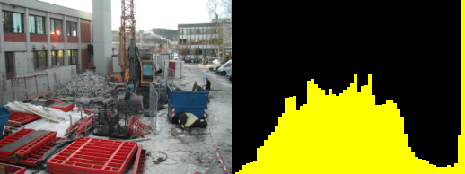
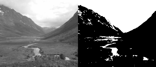
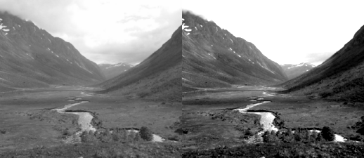
A histogram shows the distribution of low/high (dark/light) samples within an image.
The bars in the left portion of the histogram shows the amount of dark/shadow samples in the image, in the middle the mid-tones are shown and to the right the highlights.
A low contrast image will have a histogram concentrated around the middle. A dark image will have most of the histogram to the right, a bright image uses mostly the right hand side of the histogram, while a high contrast image will have few mid-tone values; making the histogram have an U shape.
The histogram in Figure 3.1, “histogram” spans from left to right, so it makes good use of the available contrast. The image is overexposed beyond repair, this can be seen from the clipping at the right hand (highlight side). This means details of the clouds in the sky are permantently lost.
Figure 3.1. histogram
function draw_rectangle(x0,y0,x1,y1,r,g,b)
  for y=y0,y1 do for x=x0,x1 do set_rgb (x,y, r,g,b) end end
end

function draw_histogram(bins)
  local bin = {}
  for i=0,bins do
    bin[i]=0
  end
  for y=0, height-1 do
     for x=0, width-1 do
        l,a,b = get_lab (x,y)
        bin[math.floor(bins * l/100)] = bin[math.floor(bins * l/100)] + 1
     end
     progress (y/height)
  end
  max = 0
  for i=0,bins do
    if bin[i]>max then
      max=bin[i]
    end
  end
  for i=0,bins do
    draw_rectangle((width/(bins+1))*i, height-(bin[i]/max*height),
             (width/(bins+1))*(i+1), height, 1, 1, 0)
  end
end

draw_rectangle(0,0,width,height,0,0,0)
draw_histogram(64)
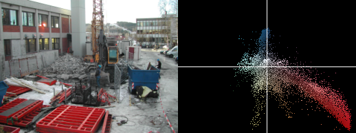
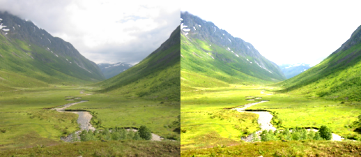
A chromaticity diagram tells us about the color distribution and saturation in an image. All pixels are plotted inside a color circle, distance to center gives saturation and angle to center specifies hue. If the white balance of an image is wrong it can most often be seen by a non centered chromaticity diagram.
| Origin in analog widget |
|---|---|
A chromaticity scope in the analog television world were traditionally created by conncting an oscilloscope to the color components of a video stream. This allowed debugging setting of the equipment handling the analog image data. | |
Figure 3.2. chromaticity diagram
function draw_rectangle(x0,y0,x1,y1,r,g,b)
  for y=y0,y1 do for x=x0,x1 do set_rgb (x,y, r,g,b) end end
end

function draw_chromascope(scale)
  if width > height then
     scale = (scale * 100)/height
  else
     scale = (scale * 100)/width
  end
  for y=0, height-1 do
     for x=0, width-1 do
        l,a,b = get_lab (x,y)
        set_lab ( (a * scale) + width*0.5,
                  (b * scale) + height*0.5,
                   l,a,b)
     end
     progress (y/height)
  end
end

draw_rectangle(0,0,width,height,0,0,0)
draw_chromascope(4)
draw_rectangle(width*0.5,0,width*0.5,height,1,1,1)
draw_rectangle(0,height*0.5,width,height*0.5,1,1,1)
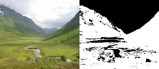
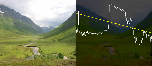
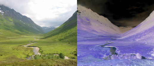
A luminiosity profile is the visualization of the luminance along a straight line in the image. The luminance plot allows a more direct way to inspect the values of an image than a histogram does.
In Figure 3.3, “luminance profile” the yellow curve indicates which line the profile is taken from, the brightness of the snow as well as the relative brightness of the sky compared to the mountains is quite apparent.
Figure 3.3. luminance profile
function draw_rectangle(x0,y0,x1,y1,r,g,b)
  for y=y0,y1 do for x=x0,x1 do set_rgb (x,y, r,g,b) end end
end

function lerp(v0,v1,r)
  return v0*(1.0-r)+v1*r
end

function draw_line(x0,y0,x1,y1,r,g,b)
  for t=0,1.0,0.001 do
    x = lerp(x0,x1,t)
    y = lerp(y0,y1,t)
    set_rgb (x,y,r,g,b)
  end
end

function lumniosity_profile(x0,y0,x1,y1)
  for y=0,height-1 do
    for x=0,width-1 do
       l,a,b = get_lab (x,y)
       set_lab (x,y, l*0.3,a,b)
    end
  end
  draw_line(x0,y0,x1,y1,1,1,0)
  prev_x, prev_y = -5, height*0.5
  for x=0,width do
     xsrc = lerp(x0,x1, x/width)
     ysrc = lerp(y0,y1, x/width)
     l,a,b = get_lab (xsrc,ysrc)
     y = height - (l/100) * height
     draw_line (prev_x, prev_y, x,y, 1,1,1)
     prev_x, prev_y = x, y
  end
end

lumniosity_profile(0,height*0.2, width,height*0.5)
“He told him, point for point, in short and plain.”
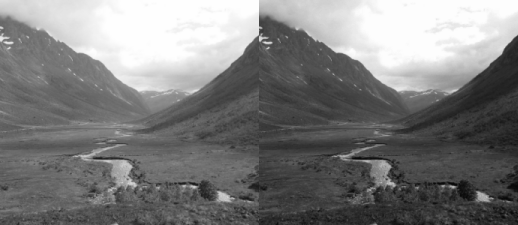
The simplest image filters are point operations, where the new value of a pixel are only determined by the original value of that single pixel alone.
Thresholding an image is the process of making all pixels above a certain threshold level white, others black.
Figure 4.1. threshold
function threshold_transform(value, level)
  if value>level then
    return 1
  else
    return 0
  end
end

function threshold_get_value(x,y,level)
  value = get_value(x,y)
  return threshold_transform(value,level)
end

function threshold(level)
   for y=0, height-1 do
     for x=0, width-1 do
       set_value (x,y, threshold_get_value(x,y,level))
     end
     progress(y/height)
   end
   flush()
end

threshold(0.5)
| Note |
|---|---|
In Figure 4.1, “threshold” and other examples for point operations, there is more code than strictly neccesary to implement the effect. The additional structuring and modularization of the code is meant to make the actual transformation of the pixel values easier to see seperated from the loops and details of dealing with the pixel data. | |
When changing the brightness of an image, a constant is added or subtracted from the luminnance of all sample values. This is equivalent to shifting the contents of the histogram left (subtraction) or right (addition).
new_value = old_value + brightness
The goal of the code in Figure 4.2, “brightness” is to add a constant amount of light to the sample value in each position in the image raster.
Figure 4.2. brightness
function add_transform(value, shift)
  return value+shift
end

function add_get_value(x,y,shift)
  value = get_value(x,y)
  return add_transform(value,shift)
end

function add(shift)
   for y=0, height-1 do
     for x=0, width-1 do
       set_value (x,y, add_get_value(x,y,shift))
     end
     progress(y/height)
   end
   flush()
end

add(0.25)
Figure 4.3. brightness subtraction
function add_transform(value, shift)
  return value+shift
end

function add_get_value(x,y,shift)
  value = get_value(x,y)
  return add_transform(value,shift)
end

function add(shift)
   for y=0, height-1 do
     for x=0, width-1 do
       set_value (x,y, add_get_value(x,y,shift))
     end
     progress(y/height)
   end
   flush()
end

function subtract(shift)
  add(-shift)
end

subtract(0.25)
Changing the contrast of an image, changes the range of luminance values present. Visualized in the histogram it is equivalent to expanding or compressing the histogram around the midpoint value. Mathematically it is expressed as:
new_value = (old_value - 0.5) × contrast + 0.5
Figure 4.4. contrast
function mul_transform(value, factor)
  return (value-0.5)*factor + 0.5
end

function mul_get_value(x,y,factor)
  value = get_value(x,y)
  return mul_transform(value,factor)
end

function mul(factor)
   for y=0, height-1 do
     for x=0, width-1 do
       set_value (x,y, mul_get_value(x,y,factor))
     end
     progress(y/height)
   end
   flush()
end

mul(2.0)
The subtraction and addition of 0.5 is to center the expansion/compression of the range around 50% gray.
Specifying a value above 1.0 will increase the contrast by making bright samples brighter and dark samples darker thus expanding on the range used. While a value below 1.0 will do the opposite and reduce use a smaller range of sample values.
It is common to bundle brightness and control in a single operations, the mathematical formula then becomes:
new_value = (old_value - 0.5) × contrast + 0.5 + brightness
Figure 4.5. brightness and contrast
function transform(value, brightness, contrast)
  return (value-0.5)*contrast+0.5+brightness
end

function transform_rgb(r,g,b, brightness, contrast)
  return transform(r, brightness, contrast), transform(g, brightness, contrast), transform(b, brightness, contrast)
end

function bcontrast_get_rgb(x,y,brightness, contrast)
   r,g,b=get_rgb(x,y)
   return transform_rgb(r,g,b, brightness, contrast)
end

function bcontrast(brightness, contrast)
    for y=0, height-1 do
      for x=0, width-1 do
        set_rgb(x,y, bcontrast_get_rgb(x,y,brightness,contrast))
      end
    end
    flush ()
end

bcontrast(0.25, 2.0)
Inverting the sample values in the image, produces the same image that would be found in a film negative. Figure 4.6, “invert”
Figure 4.6. invert
function invert_value(value)
  return 1.0-value
end

function invert_rgb(r,g,b)
  return invert_value(r),
         invert_value(g),
         invert_value(b)
end

function invert_get_rgb(x,y)
  r,g,b=get_rgb(x,y)
  return invert_rgb(r,g,b)
end

function invert()
  for y=0, height-1 do
    for x=0, width-1 do
      set_rgb(x,y, invert_get_rgb(x,y))
    end
  end
  flush()
end

invert()
A CRT monitor doesn't have a linear correspondence between the voltage sent to the electron guns and the brightness shown. The relationship is closely modelled by a powerfunction i.e. display_intensity=pixel_valuegamma. To correct an image for display, assuming the monitor doesn't already have global corrections in place. Will involve applying the function new_value=old_value1.0-gamma.
Figure 4.7. gamma
function gamma_transform(value, param)
  return value^param
end

function gamma_get_value(x,y,param)
  value = get_value(x,y)
  return gamma_transform(value,param)
end

function gamma(param)
   for y=0, height-1 do
     for x=0, width-1 do
       set_value (x,y, gamma_get_value(x,y,param))
     end
     progress(y/height)
   end
   flush()
end

gamma(1.5)
The levels tool found in many image processing packages is in it's simplest form just a different way to adjust brightness/ contrast.
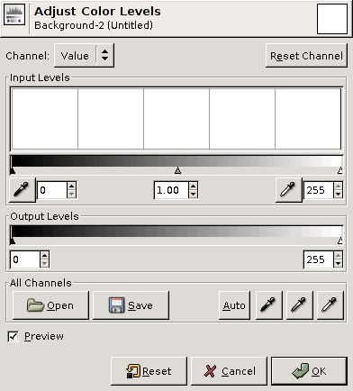
The parameters found in levels tools are in the order of spatial placement in dialogs like Figure 4.8, “The GIMP's levels tool”:
- input blacklevel
- input whitelevel
- output blacklevel
- output whitelevel
- gamma correction
Figure 4.9. levels
function levels_value(value, in_min, gamma, in_max, out_min, out_max)
  -- normalize
  value = (value-in_min) / (in_max-in_min)
  -- transform gamma
  value = value^gamma
  -- rescale range
  return value * (out_max-out_min) + out_min
end

function levels_rgb(r,g,b, in_min, gamma, in_max, out_min, out_max)
  return levels_value(r, in_min, gamma, in_max, out_min, out_max),
         levels_value(g, in_min, gamma, in_max, out_min, out_max),
         levels_value(b, in_min, gamma, in_max, out_min, out_max)
end

function levels_get_rgb(x,y, in_min, gamma, in_max, out_min, out_max)
  r,g,b=get_rgb(x,y)
  return levels_rgb(r,g,b, in_min, gamma, in_max, out_min, out_max)
end

function levels(in_min, gamma, in_max, out_min, out_max)
  for y=0, height-1 do
    for x=0, width-1 do
      set_rgb(x,y, levels_get_rgb(x,y,
         in_min, gamma, in_max,
         out_min,       out_max))
    end
  end
  flush()
end

levels(0.2, 1.2, 0.8,
       0.0,      1.2)
Figure 4.10. The GIMP's curves tool
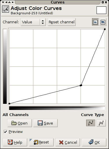
A curves filter is a filter providing the user with a free form transformation of the grayscale values in an image.
The view is a plot of the function f(x) of the transform applied, this means that the darkest values in the image are on rthe left, and the brightest on the right. The resulting value for an original value is the y value.
A diagnoal line from lower left to upper right indicates no transformation.
A horizontal line, means all pixels get the same value, along the bottom black, and along the top white.
The transform indicated in Figure 4.10, “The GIMP's curves tool” makes most values in the image darker, but allocates a larger portion of the values available to the brightest portion of the scale. This could be used to see more detail in for instance the sky in a photograph.
As can be observed in the code examples given in this chapter, there is direct mapping between input pixel values and output pixel values for point process operations.
When dealing with 8bit images, the number of input and output values are greatly reduced, if the processing taking place within the transform is expensive, having a precalculated table for all input values is a common optimizations, this is called a LookUpTable (LUT).
When the sample values stored are 16bit the advantage of a lookup table is still present since the number of entries is 65536, but when moving to 32bit floating point, the number of precalculated values needed is exceedingly large.
These exercies are not just exercies for the point operation topic, but intended as initial experiments with the gluas framework.
Write a gluas program that exchanges the red and green component of all pixels in an image.
Is this a point operation?
Create a program performing the transformation in Figure 4.10, “The GIMP's curves tool”.
Create a program that draws a 8x8 checker board on top of the existing image. The checker board should be black and white, square, cover as large area as possible and be centered on the image.
“If thence he 'scappe, into whatever world, Or unknown region.”
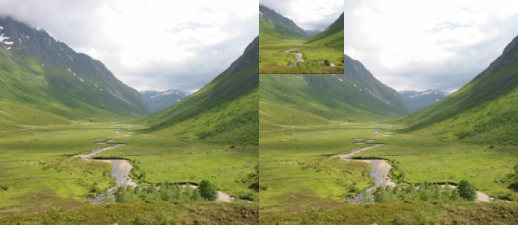
In Chapter 4, Point operations we looked at operations that calculated the new sample values of a pixel based on the value of the original pixel alone. In this chapter we look at the extension of that concept, operations that take their input from a local neighbourhood of the original pixel.
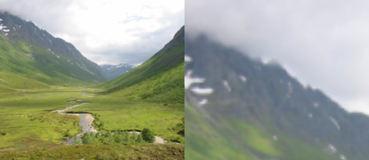
We can sample with different input windows the most common are a square or circle centered on the pixel as shown in Figure 5.1, “Sliding window”.
Figure 5.1. Sliding window
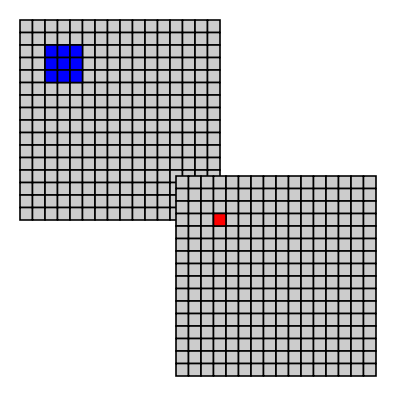
When sampling a local area around a pixel, we need to decide what to do when part of the sampling window is outside the source image. The common way to provide a "fake" value for data outside the image are:
- Make them transparent.
- Give them a color (for instance black).
- Nearest valid pixel.
- Mirror the image over the edge.
- Wrap to other side of image.
In gluas the global variable edge_duplicate can be set to 1, this makes gluas return the nearest valid pixel instead of transparent/black.
A special group of operations are the kernel filters, which use a table of numbers (a matrix) as input. The matrix gives us the weight to be given each input sample. The matrix for a kernel filter is always square and the number of rows/columns are odd. Many image filters can be expressed as convolution filters some are listed in the sourcelisting in Figure 5.3, “convolve”.
Each sample in the sampling window is weighted with the corresponding weight in the convolution matrix. The resulting sum is divided by the divisor (for most operations this is assumed to be the sum of the weights in the matrix). And finally an optional offset might be added to the result.
Figure 5.3. convolve
-- 3x3 convolution filter

edge_duplicate=1;

function convolve_get_value (x,y, kernel, divisor, offset)
   local i, j, sum
   sum_r = 0
   sum_g = 0
   sum_b = 0

   for i=-1,1 do
      for j=-1,1 do
         r,g,b = get_rgb (x+i, y+j)
         sum_r = sum_r + kernel[j+2][i+2] * r
         sum_g = sum_g + kernel[j+2][i+2] * g
         sum_b = sum_b + kernel[j+2][i+2] * b
      end
   end
   return sum_r/divisor + offset, sum_g/divisor+offset, sum_b/divisor+offset
end

function convolve_value(kernel, divisor, offset)
for y=0, height-1 do
   for x=0, width-1 do
       r,g,b = convolve_get_value (x,y, kernel, divisor, offset)
       set_rgb (x,y, r,g,b)
   end
   progress (y/height)
end
flush ()
end

function emboss()
    kernel = { { -2, -1,  0},
               { -1,  1,  1},
               {  0,  1,  2}}
    divisor = 1
    offset  = 0
    convolve_value(kernel, divisor, offset)
end

function sharpen()
    kernel = { { -1, -1, -1},
               { -1,  9, -1},
               { -1, -1, -1}}
    convolve_value(kernel, 1, 0)
end

function sobel_emboss()
    kernel = { { -1, -2, -1},
               {  0,  0,  0},
               {  1,  2,  1}}
    convolve_value(kernel, 1, 0.5)
end

function box_blur()
    kernel = { {  1,  1,  1},
               {  1,  1,  1},
               {  1,  1,  1}}
    convolve_value(kernel, 9, 0)
end

sharpen ()
A convolution matrix with all weights set to 1.0 is a blur, blurring is an operation that is often performed and can be implemented programmatically faster than the general convolution. A blur can be seen as the average of an area, or a resampling which we'll return to in a later chapter.
Figure 5.4. blur
-- a box blur filter implemented in lua

edge_duplicate = 1;

function blur_slow_get_rgba(sample_x, sample_y, radius)
   local x,y
   local rsum,gsum,bsum,asum=0,0,0,0
   local count=0

   for x=sample_x-radius, sample_x+radius do
     for y=sample_y-radius, sample_y+radius do

       local r,g,b,a= get_rgba(x,y)

       rsum, gsum, bsum, asum = rsum+r, gsum+g, bsum+b, asum+a

       count=count+1
     end
   end
   return rsum/count, gsum/count, bsum/count, asum/count
end

function blur_slow(radius)
    local x,y


    for y = 0, height-1 do
        for x = 0, width-1 do
           set_rgba (x,y, blur_slow_get_rgba (x,y,radius))
        end
        progress (y/height)
    end
    flush ()
end


-- seperation into two passes, greatly increases the speed of this
-- filter

function blur_h_get_rgba(sample_x, sample_y, radius)
   local x,y
   local rsum,gsum,bsum,asum=0,0,0,0
   local count=0

   y=sample_y
   for x=sample_x-radius, sample_x+radius do
       local r,g,b,a= get_rgba(x,y)

       rsum, gsum, bsum, asum = rsum+r, gsum+g, bsum+b, asum+a

       count=count+1
   end
   return rsum/count, gsum/count, bsum/count, asum/count
end

function blur_v(radius)
    for y = 0, height-1 do
        for x = 0, width-1 do
           set_rgba (x,y, blur_v_get_rgba(x,y,radius))
        end
        progress(y/height)
    end
    flush()
end

function blur_v_get_rgba(sample_x, sample_y, radius)
   local x,y
   local rsum,gsum,bsum,asum=0,0,0,0
   local count=0

   x=sample_x
   for y=sample_y-radius, sample_y+radius do
       local r,g,b,a= get_rgba(x,y)

       rsum, gsum, bsum, asum = rsum+r, gsum+g, bsum+b, asum+a

       count=count+1
   end
   return rsum/count, gsum/count, bsum/count, asum/count
end

function blur_h(radius)
    for y = 0, height-1 do
        for x = 0, width-1 do
           set_rgba (x,y, blur_h_get_rgba(x,y,radius))
        end
        progress(y/height)
    end
    flush()
end

function blur_fast(radius)
  blur_v(radius)
  blur_h(radius)
end

blur_fast(4)
A better looking blur is achieved by setting the weights to a gaussian distribution around the active pixel.
A gaussian blur works by weighting the input pixels near the center of ther sampling window higher than the input pixels further away.
One way to approximate a small gaussian blur, is to set the center pixel in a 3×3 matrix to 2, while the surrounding are set to 1, and set the weight to 10.
A blur is a time consuming operation especially if the radius is large. A way to optimize a blur is to observe that first blurring horizontally and then vertically gives the same result as doing both at the same time. This has been done to the blur_fast in Figure 5.4, “blur” and can also be done for gaussian blurs.
The kuwahara filter is an edge preserving blur filter. It works by calculating the mean and variance for four subquadrants, and chooses the mean value for the region with the smallest variance.
Figure 5.5. kuwahara
-- Kuwahara filter
--
--
-- Performs the Kuwahara Filter. This filter is an edge-preserving filter.
--
--
-- ( a  a  ab   b  b)
-- ( a  a  ab   b  b)
-- (ac ac abcd bd bd)
-- ( c  c  cd   d  d)
-- ( c  c  cd   d  d)
--
-- In each of the four regions (a, b, c, d), the mean brightness and the variance are calculated. The
-- output value of the center pixel (abcd) in the window is the mean value of that region that has the
-- smallest variance.
--
-- description copied from http://www.incx.nec.co.jp/imap-vision/library/wouter/kuwahara.html
--
-- implemented by Øyvind Kolås <oeyvindk@hig.no> 2004


-- the sampling window is:  width=size*2+1  height=size*2+1

size = 4

edge_duplicate = 1;

-- local function to get the mean value, and
-- variance from the rectangular area specified
function mean_and_variance (x0,y0,x1,y1)
 local variance
 local mean

 local min         = 1.0
 local max         = 0.0
 local accumulated = 0
 local count       = 0

 local x, y

 for y=y0,y1 do
   for x=x0,x1 do
     local v = get_value(x,y)

     accumulated   = accumulated + v
     count         = count + 1

     if v<min then min = v end
     if v>max then max = v end

    end
  end

  variance = max-min
  mean     = accumulated /count

  return mean, variance
end

-- local function to get the mean value, and
-- variance from the rectangular area specified
function rgb_mean_and_variance (x0,y0,x1,y1)
 local variance
 local mean
 local r_mean
 local g_mean
 local b_mean

 local min           = 1.0
 local max           = 0.0
 local accumulated_r = 0
 local accumulated_g = 0
 local accumulated_b = 0
 local count         = 0

 local x, y

 for y=y0,y1 do
   for x=x0,x1 do
     local v     = get_value(x,y)
     local r,g,b = get_rgb (x,y)

     accumulated_r   = accumulated_r + r
     accumulated_g   = accumulated_g + g
     accumulated_b   = accumulated_b + b
     count         = count + 1

     if v<min then min = v end
     if v>max then max = v end

    end
  end

  variance = max-min
  mean_r   = accumulated_r /count
  mean_g   = accumulated_g /count
  mean_b   = accumulated_b /count

  return mean_r, mean_g, mean_b, variance
end

-- return the kuwahara computed value
function kuwahara(x, y, size)
  local best_mean     = 1.0
  local best_variance = 1.0

  local mean, variance

  mean, variance = mean_and_variance (x-size, y-size, x, y)

  if variance < best_variance then
    best_mean     = mean
    best_variance = variance
  end

  mean, variance = mean_and_variance (x, y-size, x+size,y)

  if variance < best_variance then
    best_mean     = mean
    best_variance = variance
  end

  mean, variance = mean_and_variance (x, y, x+size, y+size)

  if variance < best_variance then
    best_mean     = mean
    best_variance = variance
  end

  mean, variance = mean_and_variance (x-size, y, x,y+size)

  if variance < best_variance then
    best_mean     = mean
    best_variance = variance
  end

  return best_mean
end


-- return the kuwahara computed value
function rgb_kuwahara(x, y, size)
  local best_r, best_g, best_b
  local best_variance = 1.0

  local r,g,b, variance

  r,g,b, variance = rgb_mean_and_variance (x-size, y-size, x, y)

  if variance < best_variance then
    best_r, best_g, best_b = r, g, b

    best_variance = variance
  end

  r,g,b, variance = rgb_mean_and_variance (x, y-size, x+size,y)

  if variance < best_variance then
    best_r, best_g, best_b = r, g, b
    best_variance = variance
  end

  r,g,b, variance = rgb_mean_and_variance (x, y, x+size, y+size)

  if variance < best_variance then
    best_r, best_g, best_b = r, g, b
    best_variance = variance
  end

  r,g,b, variance = rgb_mean_and_variance (x-size, y, x,y+size)

  if variance < best_variance then
    best_r, best_g, best_b = r, g, b
    best_variance = variance
  end

  return best_r, best_g, best_b
end

function kuwahara(radius)
  for y=0, height-1 do
    for x=0, width-1 do
      r,g,b = rgb_kuwahara (x,y, radius)
      set_rgb (x,y, r,g,b)
    end
    progress (y/height)
  end
end

kuwahara(2)
Rank filters operate statistically on the neighbourhood of a pixel. The tree most common rank filters are median, minimum, maximum.
The median filter sorts the sample values in theneighbourhood, and then picks the middle value. The effect is that noise is removed while detail is kept. See also kuwahara. The median filter in The GIMP is called Despeckle [5].
Figure 5.6. median
-- a median rank filter

edge_duplicate = 1;

function median_value(sample_x, sample_y, radius)
   local x,y
   local sample = {}
   local samples = 0

   for x=sample_x-radius, sample_x+radius do
     for y=sample_y-radius, sample_y+radius do

       local value = get_value(x,y)

       sample[samples] = value
       samples = samples + 1
     end
   end

   table.sort (sample)
   local mid = math.floor(samples/2)
   if math.mod(samples,2) == 1 then
       median = sample[mid+1]
   else
       median = (sample[mid]+sample[mid+1])/2
   end

   return median
end

function median(radius)
    local x,y

    for y = 0, height-1 do
        for x = 0, width-1 do
           set_value (x,y, median_value (x,y,radius))
        end
        progress (y/height)
    end
    flush ()
end

median(3)
Unsharp mask is a quite novel way to sharpen an image, it has it's origins in darkroom work. And is a multistep process.
create a duplicate image
blur the duplicate image
calculate the difference between the blurred and the original image
add the difference to the original image
The unsharp mask process works by exaggerating the mach band effect [6].
In this section some stranger filters are listed, these filters are not standard run of the mill image filters.
Pick an a random pixel within the sampling window.
Figure 5.7. jitter
-- a jittering filter implemented in lua

edge_duplicate=1 -- set edge wrap behavior to use nearest valid sample

function jitter(amount)
  local x,y
  var2=var1
  for y = 0, height-1 do
    for x = 0, width-1 do
      local nx,ny
      local r,g,b,a
      nx=x+(math.random()-0.5)*amount
      ny=y+(math.random()-0.5)*amount
      r,g,b,a=get_rgba(nx,ny)
      set_rgba(x,y, r,g,b,a)
    end
    progress(y/height)
  end
end

jitter(10)
Extend the convolve example, making it possible for it to accept a 7×7 matrix for it's values, add automatic summing to find the divisor and experiment with various sampling shapes.
Create a filter that returns the original pixel value if the variance of the entire sample window is larger than a provided value. How does this operation compare to kuwahara?
[5] The despeckle filter for gimp is more advanced than a simple median filter, it also allows for being adaptive doing more work in areas that need more work, it can be set to work recursivly. For normal median operation adaptive and recursive should be switched off, the black level set to -1 and the white level to 256.
“I want friends to motion such matter.”
Up until now, the image has remained in a fixed position, in this chapter we take a look at how we can start repositioning samples.
Affine transformations are transformations to an image that preserves colinearity, all points on a line remains on a line after transformation. Usually affine transformations are expressed as an matrices, in this text to keep the math level down, I will use geometry and vectors instead.
Translation can be described as moving the image, e.g. move all the contents of the image 50pixels to the right and 50pixels down.
Instead of traversing the original image, and placing the pixels in their new location we calculate which point in the source image ends up at the coordinate calculated.
Rotation is implemented by rotating the unit vectors of the coordinate system, and from the unit vectors calculate the new positions of a given input coordinate, to make the transformation happen in reverse it is enough to negate the angle being passed to our function.
Figure 6.2. rotation
function rotate(angle)
  for y=0, height-1 do
    for x=0, width-1 do
      -- calculate the source coordinates (u,v)
      u = x * math.cos(-angle) + y * math.sin(-angle)
      v = y * math.cos(-angle) - x * math.sin(-angle)

      r,g,b = get_rgba(u,v)
      set_rgb(x,y,r,g,b)
    end
    progress (y/height)
  end
  flush()
end

rotate(math.rad(15))
Scaling an image is a matter of scaling both the x and y axes according to a given scale factor when retrieving sample values.

Perspective transformations are useful for texture mapping, texture mapping is outside the scope of this text. Affine transformations are a subset of perspective transformations.
To be able to do texturemapping for use in realtime 3d graphics, the algorithm is usually combined with a routine that only paints values within the polygon defined, such a routine is called a polyfiller.
When doing stitching of individual images to create a larger image, correction for the lens is needed, the only difference compared to the earlier mentioned affine transformations are that the parameters used to calculate the distortion are based on properties of the lens.
When doing rotation as well as scaling, the coordinates we end up getting pixel values from are not neccesary integer coordinates. When enlarging this problem is especially apparent in Figure 6.3, “scaling” the problem is quite apparent we have "enlarged" each sample (pixel) to cover a larger area, this results in blocky artifacts within the image.
A more correct approach is to make an eduacted guess about the missing value at the sampling coordinates, this means attempting to get the results we would have gotten by sampling that coordinate in the original continous analog image plane.
The method used in the affine samples above is called "nearest neighbour", getting the closest corresponding pixel in the source image.
Bilinear sampling makes the assumption that values in the image changes continously.
Figure 6.4. bilinear
function get_rgb_bilinear (x,y)
  local x0,y0 -- integer coordinates
  local dx,dy -- offset from coordinates
  local r0,g0,b0, r1,g1,b1, r2,g2,b2, r3,g3,b3
  local r,g,b

  x0=math.floor(x)
  y0=math.floor(y)
  dx=x-x0
  dy=y-y0

  r0,g0,b0 = get_rgb (x0  ,y0  )
  r1,g1,b1 = get_rgb (x0+1,y0  )
  r2,g2,b2 = get_rgb (x0+1,y0+1)
  r3,g3,b3 = get_rgb (x0  ,y0+1)

  r = lerp (lerp (r0, r1, dx), lerp (r3, r2, dx), dy)
  g = lerp (lerp (g0, g1, dx), lerp (g3, g2, dx), dy)
  b = lerp (lerp (b0, b1, dx), lerp (b3, b2, dx), dy)

  return r,g,b
end

function scale(ratio)
  for y=0, height-1 do
    for x=0, width-1 do
      -- calculate the source coordinates (u,v)
      u = x * (1.0/ratio)
      v = y * (1.0/ratio)
      r,g,b=get_rgb_bilinear(u,v)
      set_rgb(x,y,r,g,b)
    end
    progress (y/height)
  end
  flush()
end

function lerp(v1,v2,ratio)
   return v1*(1-ratio)+v2*ratio;
end
-- LERP
-- /lerp/, vi.,n.
--
-- Quasi-acronym for Linear Interpolation, used as a verb or noun for
-- the operation. "Bresenham's algorithm lerps incrementally between the
-- two endpoints of the line." (From Jargon File (4.4.4, 14 Aug 2003)
scale(3)
Figure 6.5. bicubic

function get_rgb_cubic_row(x,y,offset)
  local r0,g0,b0, r1,g1,b1, r2,g2,b2, r3,g3,b3
  r0,g0,b0 = get_rgb(x,y)
  r1,g1,b1 = get_rgb(x+1,y)
  r2,g2,b2 = get_rgb(x+2,y)
  r3,g3,b3 = get_rgb(x+3,y)
  return cubic(offset,r0,r1,r2,r3), cubic(offset,g0,g1,g2,g3), cubic(offset,b0,b1,b2,b3)
end

function get_rgb_bicubic (x,y)
  local xi,yi -- integer coordinates
  local dx,dy -- offset from coordinates
  local r,g,b

  xi=math.floor(x)
  yi=math.floor(y)
  dx=x-xi
  dy=y-yi

  r0,g0,b0 = get_rgb_cubic_row(xi-1,yi-1,dx)
  r1,g1,b1 = get_rgb_cubic_row(xi-1,yi,  dx)
  r2,g2,b2 = get_rgb_cubic_row(xi-1,yi+1,dx)
  r3,g3,b3 = get_rgb_cubic_row(xi-1,yi+2,dx)

  return cubic(dy,r0,r1,r2,r3),
         cubic(dy,g0,g1,g2,g3),
         cubic(dy,b0,b1,b2,b3)
end

function scale(ratio)
  for y=0, height-1 do
    for x=0, width-1 do
      -- calculate the source coordinates (u,v)
      u = x * (1.0/ratio)
      v = y * (1.0/ratio)
      r,g,b=get_rgb_bicubic(u,v)
      set_rgb(x,y,r,g,b)
    end
    progress (y/height)
  end
  flush()
end

function cubic(offset,v0,v1,v2,v3)
  -- offset is the offset of the sampled value between v1 and v2
   return   (((( -7 * v0 + 21 * v1 - 21 * v2 + 7 * v3 ) * offset +
               ( 15 * v0 - 36 * v1 + 27 * v2 - 6 * v3 ) ) * offset +
               ( -9 * v0 + 9 * v2 ) ) * offset + (v0 + 16 * v1 + v2) ) / 18.0;
end

scale(3)
When scaling an image down the output contains fewer pixels (sample points) than the input. We are not guessing the value of in-between locations, but combining multiple input pixels to a single output pixel.
One way of doing this is to use a box filter and calculate a weighted average of the contribution of all pixel values.
Figure 6.6. box decimate
function get_rgb_box(x0,y0,x1,y1)
  local area=0 -- total area accumulated in pixels
  local rsum,gsum,bsum = 0,0,0
  local x,y
  local xsize, ysize

  for y=math.floor(y0),math.ceil(y1) do
    ysize = 1.0
    if y<y0 then
      size = size * (1.0-(y0-y))
    end
    if y>y1 then
      size = size * (1.0-(y-y1))
    end
    for x=math.floor(x0),math.ceil(x1) do
      size = ysize
      r,g,b = get_rgb(x,y)
      if x<x0 then
        size = size * (1.0-(x0-x))
      end
      if x>x1 then
        size = size * (1.0-(x-x1))
      end
      rsum,gsum,bsum = rsum + r*size, gsum + g*size, bsum + b*size
      area = area+size
    end
  end

  return rsum/area, gsum/area, bsum/area
end

function scale(ratio)
  for y=0, (height*ratio)-1 do
    for x=0, (width*ratio)-1 do
      u0 = x * (1.0/ratio)
      v0 = y * (1.0/ratio)
      u1 = (x+1) * (1.0/ratio)
      v1 = (y+1) * (1.0/ratio)
      r,g,b=get_rgb_box(u0,v0,u1,v1)
      set_rgb(x,y,r,g,b)
    end
    progress (y/(height*ratio))
  end
  flush()
end

scale(0.33)
With OpenGL and other realtime 3d engines it is common to use mipmaps to increase the speed and quality of resampled textured.
A mipmap is a collection of images of prescaled sizes. The prescaled sizes are 1.0×image dimensions, 0.5×image dimensions, 0.25×image dimensions, 0.125×image dimensions etc.
When retrieving a sample value a bilinear interpolation would be performed at both the version of the image larger than the scaling ratio as well as the image smaller than the scaling ratio. After that a linear interpolation is performed on the two resulting values based on which of the two versions most closely matches the target resolution.
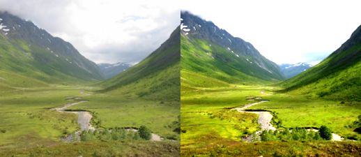
Using The GIMP open a test image, create a duplicate of the original image. (Image/Duplicate). Scale the duplicate image to 25% size (Image/Scale). Scale the duplicate image up 400%. Copy the newly scaled image as a layer on top of the original image. (Ctrl+C, change image Ctrl+V), and press the new layer button when the original image is active. Set the mode of the top layer to difference, Flatten the image (Image/Flatten Image), and automatically stretch the contrast of the image. (Layer/Colors/Auto/Stretch Contrast).
Do this for nearest neighbour, bilienar and bicubic interpolation and compare the results.
Read Appendix A, Assignment, spring 2005 and perhaps make initial attempts at demosaicing the Bayer pattern.
“Any sufficiently advanced technology is indistinguishable from magic.”
Algorithms for automatic adjustments attempts to automatically enhance the perceptual quality of an image. Such algorithms are usually used to enhance the perceived quality of images.
Digital cameras, often use such algorithms after aquisition, to make the most out of the data captured by the light sensor.
Companies providing print services for consumers, both developing analog film and scanning it; as well as companies making prints directly from digital files. The selection and tuning of parameters are based on automatically categorizing the image as a portrait, landscape, sunset/sunrise etc.
To achieve the best results possible, manual tuning and adjustments are often needed, but for a normal private use, like holiday pictures automatic enhancements makes higher quality easy, and point and shoot photography possible.
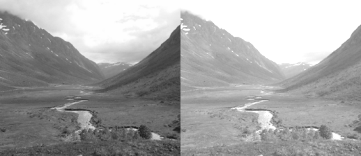
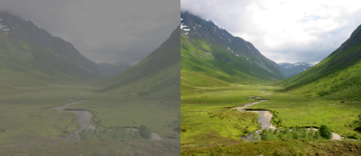
Contrast stretching makes sure the input sample with the lowest value is mapped to black; and that the one with the highest to 1.0. The values are recalculated by using linear interpolation.
Contrast stretching automatically counters under and over exposure, as well as the ability to extend the used luminance range.
It is also possible to restrict the algorithm towards the center of the distribution, perhaps with a cut-off value, this allows for a more noise tolerant adjustment.
Figure 7.1. contrast stretching
function get_min_max()
    min, max = 1000, -1000
    for y=0, height-1 do
      for x=0, width-1 do
        value = get_value(x,y)
        if value<min then
          min = value
        end
        if value>max then
          max = value
        end
      end
    end
    return min,max
end

function remap(v, min, max)
    return (v-min) * 1.0/(max-min)
end

function cs_get_rgb(x,y,min,max)
    r,g,b = get_rgb(x,y)
    r = remap(r, min, max)
    g = remap(g, min, max)
    b = remap(b, min, max)
    return r,g,b
end

function contrast_stretch()
    min, max = get_min_max()

    for y=0, height do
      for x=0, width do
        set_rgb(x,y, cs_get_rgb(x,y,min,max))
      end
    end
    flush ()
end

contrast_stretch()
In the day of analog point and shoot photography, the white balance of the images were set by the photolab. With digital photography the whitebalance has to either be pre set by the photographer by measurement or guess, or be guessed by algorithms in camera or computer software.
Assuming that we have a good distribution of colors in our scene, the average reflected color should be the color of the light. If the light source is assumed to be white, we know how much the whitepoint should be moved in the color cube.
The compensation calculated by the gray world assumption is an approximation of the measurement taken by digital still and video cameras by capturing an evenly lit white sheet of paper or similar.
Figure 7.2. grayworld assumption
function get_avg_a_b ()
    sum_a=0
    sum_b=0

    -- first find average color in CIE Lab space
    for y=0, height-1 do
      for x=0, width-1 do
        l,a,b = get_lab(x,y)
        sum_a, sum_b = sum_a+a, sum_b+b
      end
      progress(y/height)
    end

    avg_a=sum_a/(width*height)
    avg_b=sum_b/(width*height)

    return avg_a,avg_b
end

function shift_a_b(a_shift, b_shift)
    for y=0, height do
      for x=0, width do
        l,a,b = get_lab(x,y)

        -- scale the chroma distance shifted according to amount of
        -- luminance. The 1.1 overshoot is because we cannot be sure
        -- to have gotten the data in the first place.
        a_delta = a_shift * (l/100) * 1.1
        b_delta = b_shift * (l/100) * 1.1
        a,b = a+a_delta, b+b_delta

        set_lab(x,y,l,a,b)
      end
      progress(y/height)
    end
    flush()
end

function grayworld_assumption()
  avg_a, avg_b = get_avg_a_b()
  shift_a_b(-avg_a, -avg_b)
end

grayworld_assumption()
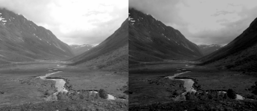
Component stretching makes the assumption that either direct reflections, or glossy reflections from surfaces can be found in the image, and that it is amongst the brightest colors in the image. By stretching each R,G and B component to it's full range, as in the section called “Contrast stretching” often leads to a better result than grayworld assumption.
If the image is overexposed, this technique does not work, not having a very reflective object will also bias the results in a non desireable way.
Figure 7.3. component stretching
function get_min_max_r ()
    min, max = 1000, -1000
    for y=0, height-1 do
      for x=0, width-1 do
        value, temp, temp = get_rgb (x,y)
        if value<min then
          min = value
        end
        if value>max then
          max = value
        end
      end
    end
    return min,max
end

function get_min_max_g ()
    min, max = 1000, -1000
    for y=0, height-1 do
      for x=0, width-1 do
        temp, value, temp = get_rgb (x,y)
        if value<min then
          min = value
        end
        if value>max then
          max = value
        end
      end
    end
    return min,max
end

function get_min_max_b ()
    min, max = 1000, -1000
    for y=0, height-1 do
      for x=0, width-1 do
        temp, temp, value = get_rgb (x,y)
        if value<min then
          min = value
        end
        if value>max then
          max = value
        end
      end
    end
    return min,max
end

function remap(v, min, max)
    return (v-min) * 1.0/(max-min)
end

function cs_get_rgb(x,y,min_r,max_r,min_g,max_g,min_b,max_b)
    r,g,b = get_rgb(x,y)
    r = remap(r, min_r, max_r)
    g = remap(g, min_g, max_g)
    b = remap(b, min_b, max_b)
    return r,g,b
end

function component_stretch()
    min_r, max_r = get_min_max_r ()
    min_g, max_g = get_min_max_g ()
    min_b, max_b = get_min_max_b ()

    for y=0, height do
      for x=0, width do
        set_rgb(x,y, cs_get_rgb(x,y,min_r,max_r, min_g, max_g, min_b, max_b))
      end
    end
    flush ()
end

component_stretch()
ACE is an algorithm that performs contrast stretching based on statistical data taken from the neighbourhood of the pixel being processed, this allows for extending the dynamic range of an image based on local features, this is a process often found useful in medical images. The algorithm makes it possible to see things hidden in darkness in one area of an image, without destroying the details in another.
Figure 7.4. ace
edge_duplicate = 1;

function get_min_max (x0,y0,x1,y1)
    min_r, max_r = 1000, -1000
    min_g, max_g = 1000, -1000
    min_b, max_b = 1000, -1000
    for y=y0,y1 do
      for x=x0,x1 do
        r, g, b= get_rgb (x,y)
        if r<min_r then min_r = r end if r>max_r then max_r = r end
        if g<min_g then min_g = g end if g>max_g then max_g = g end
        if b<min_b then min_b = b end if b>max_b then max_b = b end
      end
    end
    return min_r,max_r,min_g,max_g,min_b,max_b
end

function remap(v, min, max)
    return (v-min) * 1.0/(max-min)
end

function ace_get_rgb(x,y,radius)
    min_r, max_r, min_g, max_g, min_b, max_b =
          get_min_max (x-radius,y-radius,x+radius,y+radius)
    r,g,b = get_rgb(x,y)
    r = remap(r, min_r, max_r)
    g = remap(g, min_g, max_g)
    b = remap(b, min_b, max_b)
    return r,g,b
end

function ace(radius)

    for y=0, height do
      for x=0, width do
        set_rgb(x,y, ace_get_rgb(x,y,radius))
      end
      progress (y/height)
      print (y/height)
    end
    flush ()
end

ace(32)
| Note |
|---|---|
This implementation of ACE doesn't really show the potential of the algorithm, a better test image, and an implementation that has received more care would be preffered, see also exercise 1. | |
The artifacts appearing in Figure 7.4, “ace” are due to the sampling of the pixels used to find the maximum and minimum values to do contrast stretching with. How can the ACE filter be improved to give a smoother appearance?
Artifact: Technology an object, oservation, phenomenon, or result arising from hidden or unexpected causes extraneous to the subject of a study, and therefore spurious and having potential to lead one to an erroneous conclusion, or to invalidate the study. In experimental science, artifacts may arise due to inadvertant contamination of equipment, faulty experimental design or faulty analysis, or unexpected effects of agencies not known to affect the system under study.
Some sensors have permanently stuck pixels, or pixels that have a different sensitivity than others. This is a problem that can be fixed by having a "blank" exposure that records the difference between pixels. The pattern found by taking this blank shot can be used to correct both the intensity of recorded values, as well as replacing known to be bad pixels.
Some digital cameras keep a track of bad pixels themselves, when getting a RAW file, the bad pixels are usually not retouched.
Analog film effectivly has many small light sensitive particles that act as sensors. With fast films, that need little light, the density of these particles is low, which lead to a grainy texture on the images.
Film grain is countered by various lowpass filters, like blurring and median. Other more advanced filters reconstructs vector fields of "flow" in the image.
Note that sometimes the goal is to create noise to match original film grain, this can be achieved by analysis of blank frames of video to extract patterns with statistical properties similar to the film-grain.
CCD's have the same problems as physical film except the noise appears to be even more random. CCD noise is more statistically uniform and thus can be quite well countered with a median filter.
The quantification process can introducate artifacts. Increase in contrast and colorspace conversions can amplify quantification artifacts. The old adage, GIGO, Garbage In, Garbage Out. there isn't very much to do with data that is bad from the outset.
Old analog TV equipment did a neat trick to allow for both a high temporal rate as well as a high number of lines. Only every second line were transmitted, first the odd lines, then the even lines. This way of displaying images only work well for CRT monitors. For LCDs an interlaced image must be resampled to avoid combing artifacts.
Line doubling is the simplest form of deinterlacing, it replaces the odd lines with the even lines. This gets rid of the interlacing effect, but reduces the vertical resolution in half.
"Linear Blend operates by taking a line, then averaging the pixel values in it with the line below, effectively blurring the frame. This almost completely eliminates the effects of interlacing - at times you may notice slight ghosting (instant transition from one thing to another), the image appears to persist for a fraction of a second. This is absolutely not a serious issue, as far as I am concerned - in fact it's really only noticeable if you are me, and a perfectionist." [quote from http://xaw-deinterlace.sourceforge.net/index.php?sec=about]
By reconstructing motion vectors for the video frames, it is possible to predict the position of object between frames, thus providing a volume video object where any position can be sampled. Such an advanced approach can be used for both deinterlacing and high quality time stretching.
Aliasing artifacts, result from a spatial sampling frequency that is too low. A common example is moire effect showing up on textiles, like tweed, with detailed repeating patterns like tweed.
One way to counter aliasing is blurring the image. If we have control over the creation of the problematic image, we can also render a high resolution version that is downsampled to the target resolution using decimation.
You are to implement a program that takes the data from the CMOS sensor, and generates an as good RGB image as possible.
You will write a short report about the strategy taken and how you have implemented it, the report shall be delvivered as a zipped folder through classfronter. The zip file should contain the source code for your implementation, an index.html file containing the main text of the report as well as the result of running your algorithm on 3 or more of the given sample images.
Your images should attempt creating as good color images as possible from the following Bayer pattern screened grayscale images.