“He told him, point for point, in short and plain.”
The simplest image filters are point operations, where the new value of a pixel are only determined by the original value of that single pixel alone.
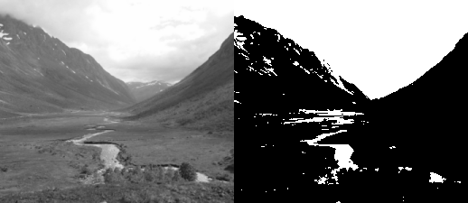
Thresholding an image is the process of making all pixels above a certain threshold level white, others black.
Figure 4.1. threshold
function threshold_transform(value, level)
  if value>level then
    return 1
  else
    return 0
  end
end

function threshold_get_value(x,y,level)
  value = get_value(x,y)
  return threshold_transform(value,level)
end

function threshold(level)
   for y=0, height-1 do
     for x=0, width-1 do
       set_value (x,y, threshold_get_value(x,y,level))
     end
     progress(y/height)
   end
   flush()
end

threshold(0.5)
![[Note]](images/note.png) | Note |
|---|---|
In Figure 4.1, “threshold” and other examples for point operations, there is more code than strictly neccesary to implement the effect. The additional structuring and modularization of the code is meant to make the actual transformation of the pixel values easier to see seperated from the loops and details of dealing with the pixel data. |
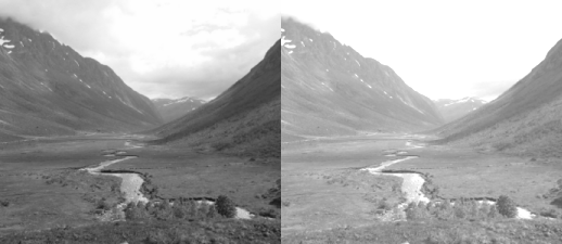
When changing the brightness of an image, a constant is added or subtracted from the luminnance of all sample values. This is equivalent to shifting the contents of the histogram left (subtraction) or right (addition).
new_value = old_value + brightness
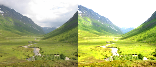
The goal of the code in Figure 4.2, “brightness” is to add a constant amount of light to the sample value in each position in the image raster.
Figure 4.2. brightness
function add_transform(value, shift)
  return value+shift
end

function add_get_value(x,y,shift)
  value = get_value(x,y)
  return add_transform(value,shift)
end

function add(shift)
   for y=0, height-1 do
     for x=0, width-1 do
       set_value (x,y, add_get_value(x,y,shift))
     end
     progress(y/height)
   end
   flush()
end

add(0.25)
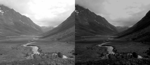
Figure 4.3. brightness subtraction
function add_transform(value, shift)
  return value+shift
end

function add_get_value(x,y,shift)
  value = get_value(x,y)
  return add_transform(value,shift)
end

function add(shift)
   for y=0, height-1 do
     for x=0, width-1 do
       set_value (x,y, add_get_value(x,y,shift))
     end
     progress(y/height)
   end
   flush()
end

function subtract(shift)
  add(-shift)
end

subtract(0.25)
Changing the contrast of an image, changes the range of luminance values present. Visualized in the histogram it is equivalent to expanding or compressing the histogram around the midpoint value. Mathematically it is expressed as:
new_value = (old_value - 0.5) × contrast + 0.5
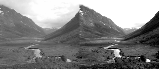
Figure 4.4. contrast
function mul_transform(value, factor)
  return (value-0.5)*factor + 0.5
end

function mul_get_value(x,y,factor)
  value = get_value(x,y)
  return mul_transform(value,factor)
end

function mul(factor)
   for y=0, height-1 do
     for x=0, width-1 do
       set_value (x,y, mul_get_value(x,y,factor))
     end
     progress(y/height)
   end
   flush()
end

mul(2.0)
The subtraction and addition of 0.5 is to center the expansion/compression of the range around 50% gray.
Specifying a value above 1.0 will increase the contrast by making bright samples brighter and dark samples darker thus expanding on the range used. While a value below 1.0 will do the opposite and reduce use a smaller range of sample values.
It is common to bundle brightness and control in a single operations, the mathematical formula then becomes:
new_value = (old_value - 0.5) × contrast + 0.5 + brightness
Figure 4.5. brightness and contrast
function transform(value, brightness, contrast)
  return (value-0.5)*contrast+0.5+brightness
end

function transform_rgb(r,g,b, brightness, contrast)
  return transform(r, brightness, contrast), transform(g, brightness, contrast), transform(b, brightness, contrast)
end

function bcontrast_get_rgb(x,y,brightness, contrast)
   r,g,b=get_rgb(x,y)
   return transform_rgb(r,g,b, brightness, contrast)
end

function bcontrast(brightness, contrast)
    for y=0, height-1 do
      for x=0, width-1 do
        set_rgb(x,y, bcontrast_get_rgb(x,y,brightness,contrast))
      end
    end
    flush ()
end

bcontrast(0.25, 2.0)
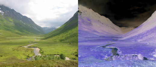
Inverting the sample values in the image, produces the same image that would be found in a film negative. Figure 4.6, “invert”
Figure 4.6. invert
function invert_value(value)
  return 1.0-value
end

function invert_rgb(r,g,b)
  return invert_value(r),
         invert_value(g),
         invert_value(b)
end

function invert_get_rgb(x,y)
  r,g,b=get_rgb(x,y)
  return invert_rgb(r,g,b)
end

function invert()
  for y=0, height-1 do
    for x=0, width-1 do
      set_rgb(x,y, invert_get_rgb(x,y))
    end
  end
  flush()
end

invert()
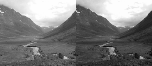
A CRT monitor doesn't have a linear correspondence between the voltage sent to the electron guns and the brightness shown. The relationship is closely modelled by a powerfunction i.e. display_intensity=pixel_valuegamma. To correct an image for display, assuming the monitor doesn't already have global corrections in place. Will involve applying the function new_value=old_value1.0-gamma.
Figure 4.7. gamma
function gamma_transform(value, param)
  return value^param
end

function gamma_get_value(x,y,param)
  value = get_value(x,y)
  return gamma_transform(value,param)
end

function gamma(param)
   for y=0, height-1 do
     for x=0, width-1 do
       set_value (x,y, gamma_get_value(x,y,param))
     end
     progress(y/height)
   end
   flush()
end

gamma(1.5)
The levels tool found in many image processing packages is in it's simplest form just a different way to adjust brightness/ contrast.
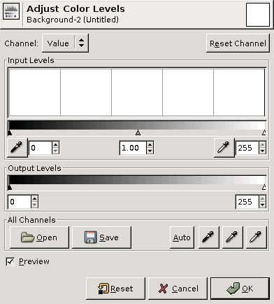
The parameters found in levels tools are in the order of spatial placement in dialogs like Figure 4.8, “The GIMP's levels tool”:
- input blacklevel
- input whitelevel
- output blacklevel
- output whitelevel
- gamma correction
Figure 4.9. levels
function levels_value(value, in_min, gamma, in_max, out_min, out_max)
  -- normalize
  value = (value-in_min) / (in_max-in_min)
  -- transform gamma
  value = value^gamma
  -- rescale range
  return value * (out_max-out_min) + out_min
end

function levels_rgb(r,g,b, in_min, gamma, in_max, out_min, out_max)
  return levels_value(r, in_min, gamma, in_max, out_min, out_max),
         levels_value(g, in_min, gamma, in_max, out_min, out_max),
         levels_value(b, in_min, gamma, in_max, out_min, out_max)
end

function levels_get_rgb(x,y, in_min, gamma, in_max, out_min, out_max)
  r,g,b=get_rgb(x,y)
  return levels_rgb(r,g,b, in_min, gamma, in_max, out_min, out_max)
end

function levels(in_min, gamma, in_max, out_min, out_max)
  for y=0, height-1 do
    for x=0, width-1 do
      set_rgb(x,y, levels_get_rgb(x,y,
         in_min, gamma, in_max,
         out_min,       out_max))
    end
  end
  flush()
end

levels(0.2, 1.2, 0.8,
       0.0,      1.2)
Figure 4.10. The GIMP's curves tool
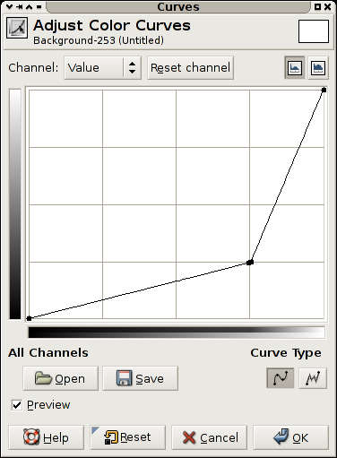
A curves filter is a filter providing the user with a free form transformation of the grayscale values in an image.
The view is a plot of the function f(x) of the transform applied, this means that the darkest values in the image are on rthe left, and the brightest on the right. The resulting value for an original value is the y value.
A diagnoal line from lower left to upper right indicates no transformation.
A horizontal line, means all pixels get the same value, along the bottom black, and along the top white.
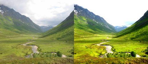
The transform indicated in Figure 4.10, “The GIMP's curves tool” makes most values in the image darker, but allocates a larger portion of the values available to the brightest portion of the scale. This could be used to see more detail in for instance the sky in a photograph.
As can be observed in the code examples given in this chapter, there is direct mapping between input pixel values and output pixel values for point process operations.
When dealing with 8bit images, the number of input and output values are greatly reduced, if the processing taking place within the transform is expensive, having a precalculated table for all input values is a common optimizations, this is called a LookUpTable (LUT).
When the sample values stored are 16bit the advantage of a lookup table is still present since the number of entries is 65536, but when moving to 32bit floating point, the number of precalculated values needed is exceedingly large.
These exercies are not just exercies for the point operation topic, but intended as initial experiments with the gluas framework.
Write a gluas program that exchanges the red and green component of all pixels in an image.
Is this a point operation?
Create a program performing the transformation in Figure 4.10, “The GIMP's curves tool”.
Create a program that draws a 8x8 checker board on top of the existing image. The checker board should be black and white, square, cover as large area as possible and be centered on the image.